We know what a zero of a function is and what a zero of an analytic function is: if  is analytic at point
  for which
  then
then  where
where  and
and  is analytic..and this decomposition is unique (via the uniqueness of a power series).
  is the order of the zero.
What I did not tell you is that a zero of a NON-CONSTANT analytic function is isolated; that is, there is some  such that: if
  is the open disk of radius
  about and
  then
then  . That is, a zero of an analytic function can be isolated from other zeros.
Here is why: Suppose not; then there is some sequence of  where
where  (how to construct: choose a zero
  to be closer than 1 to and then let
  be a zero of that is less than half the distance between and and keep repeating this process. It cannot terminate because if it does, it means that the zeros are isolated from .
Note that for  we have
  which implies that
  . But is analytic and since for all
  then
then  which contradicts the fact that . So, the zeros of an analytic function are isolated.
In fact, we can say even more (that an analytic function is a “discrete mapping”..that is, roughly speaking, takes a discrete set to a discrete set) but we’ll leave that alone, at least for now. See: Discrete Mapping Theorem in Bruce Palka’s complex variables book
But for now, we’ll just stick with this.
Note: in real analysis, there is the concept of a “bump function”: one which is zero on some interval (or region), not zero off of that region and is infinitely smooth (has derivatives of all orders). This cannot happen with analytic complex functions.
Now onto poles.
A singularity of a complex function is a point at which the complex function is not analytic. A singularity is isolated if one can put an open disk around it on which the function is analytic EXCEPT at the singularity.
More formally: say has an isolated singularity if is NOT analytic at but is analytic on some set  for some
  . (these sets are referred to as “punctured disks” or “deleted disks”. )
Example:  has an isolated singularity at
  .
.  has isolated singularities at
Example:  has isolated singularities at
  where
where  is one of the n-th roots of unity.
  has an isolated singularity at
Example:  is not analytic anywhere an therefore has no isolated singularities.
Example:  has isolated singularities at
  and has a non-isolated singularity at .
  has non isolated singularities at the origin and the negative real axis.
We will deal with isolated singularities.
There are three types:
1. Removable or “inessential”. This is the case where is technically not analytic at but  exists. Think of functions like
  etc. It is easy to see what the limits are; just write out the power series centered at and do the algebra.
What we do here is to say: if  then let
  and note that is analytic. So, it does no harm to all but ignore the inessential singularities.
2. Essential singularities: these are weird objects. Here is what I will say: has an essential singularity at  if is neither removable nor a pole. Of course, I need to tell you what a pole is.
Why these are weird: if has an essential singularity at and  is ANY punctured disk containing in its center but containing no other singularities, and
  is ANY complex number (with at most exception), then there exits
  where
where  . This is startling; this basically means that maps every punctured disk around an essential singularity to the entire complex plane, possibly minus one point. This is the Great Picard’s Theorem. (we will prove a small version of this; not the full thing).
Example:  has an essential singularity at . If this seems like an opaque claim, it will be crystal clear when we study Laurent series, which are basically power series, but possibly with terms with negative powers.
3. Poles (what we will spend our time with). If is not analytic at but there is some positive integer such that  exists, then we say that has pole of order m at .
“Easy examples”: has a pole of order 1 at the origin (called a “simple pole”).  has simple poles at
  and a pole of order 2 (called a “double pole”) at
 has a pole of order 2 at the origin. (if that seems like a strange claim, write out the power series for
  then do the division.)
Relation to zeros:
Fact: if is analytic and has a zero of order at , then  has a pole of order at .
Note: because zeros of analytic functions are isolated, the singularity of is isolated. Now:
 is analytic at (no zero in the denominator any longer). Note that is the smallest integer that works because any smaller integer would leave a zero in the denominator.
Fact: if has a pole of order at then has a zero of order at .
Reason: Let  be the associated analytic function (with m being the smallest integer that works ). Since this is the smallest that works, we can assume that (look at the power series for
  ; if the first term has
  to a non zero power, use a lower power of m )
Now  is zero at
  (denominator is not zero).
So the poles and zeros of an analytic function are very closely linked; they are basically the duals of each other. The calculus intuition of “check for zeros in the denominator” works very well here.
Onward to Laurent series and residues
Start with poles or order : If has a pole of order at then we know  is analytic on some open disk of convergence about .
So we can write  .
.
So  .
.
Now divide both sized by  and look at what happens to the series:

So while does not have a power series centered at it does have a series of a sort. Such a series is called a Laurent series. It is traditional to write:
 . Of course, for a pole of order , at most terms of the first series will have non-zero coefficients. For an essential singularity, an infinite number of the coefficients will be non-zero. We will see that the first series yields a function that is analytic for
  for some
  and the second series, a power series, is analytic within some open disk of convergence (as usual).
Terminology:  is called the principal part of the Laurent series, and
  is called the regular part.
 (the coefficient of the
  is called the residue of at
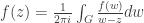
Why this is important: Let  be a small circle that encloses but no other singularities. Then
  . This is the famous Residue Theorem and this arises from simple term by term integration of the Laurent series. For a pole it is easy: the integral of the regular part is zero since the regular part is an analytic function, so we need only integrate around the terms with negative powers and there are only a finite number of these.
Each  has a primitive EXCEPT for
  so each of these integrals are zero as well. So ONLY THE term matters, with regards to integrating around a closed loop!
The proof is not quite as straight forward if the singularity is essential, though the result still holds. For example:
 but the result still holds; we just have to be a bit more careful about justifying term by term integration.
So, if is at all reasonable (only isolated singularities), then integrating along a closed curve amounts to finding the residues within the curve (and having the curve avoid the singularities, of course), adding them up and multiplying by  . Note: this ONLY applies to with isolated singularities; for other functions (say ) we have to grit our teeth a parameterize the curve the old fashioned way.
Now FINDING those residues can be easy, or at times, difficult. Stay tuned.


![[1, 4]](https://s0.wp.com/latex.php?latex=%5B1%2C+4%5D+&bg=ffffff&fg=333333&s=0&c=20201002)
